This book uses the R programming language to illustrate all concepts and examples. It assumes that readers have a basic understanding of R. However, for completeness, this chapter provides a concise introduction to key R concepts to support readers who are new to R or who would benefit from a refresher.
2.1 R basics
R is a programming language that was developed by statisticians and for statisticians. Though in modern times it has found its way into other domains like arts, the original intent of it’s developers (Rose Ihaka and Robert Gentleman) was to use it for carrying out statistical computing work. R is open source and therefore available to anyone, what you need is to download and install it on your system.
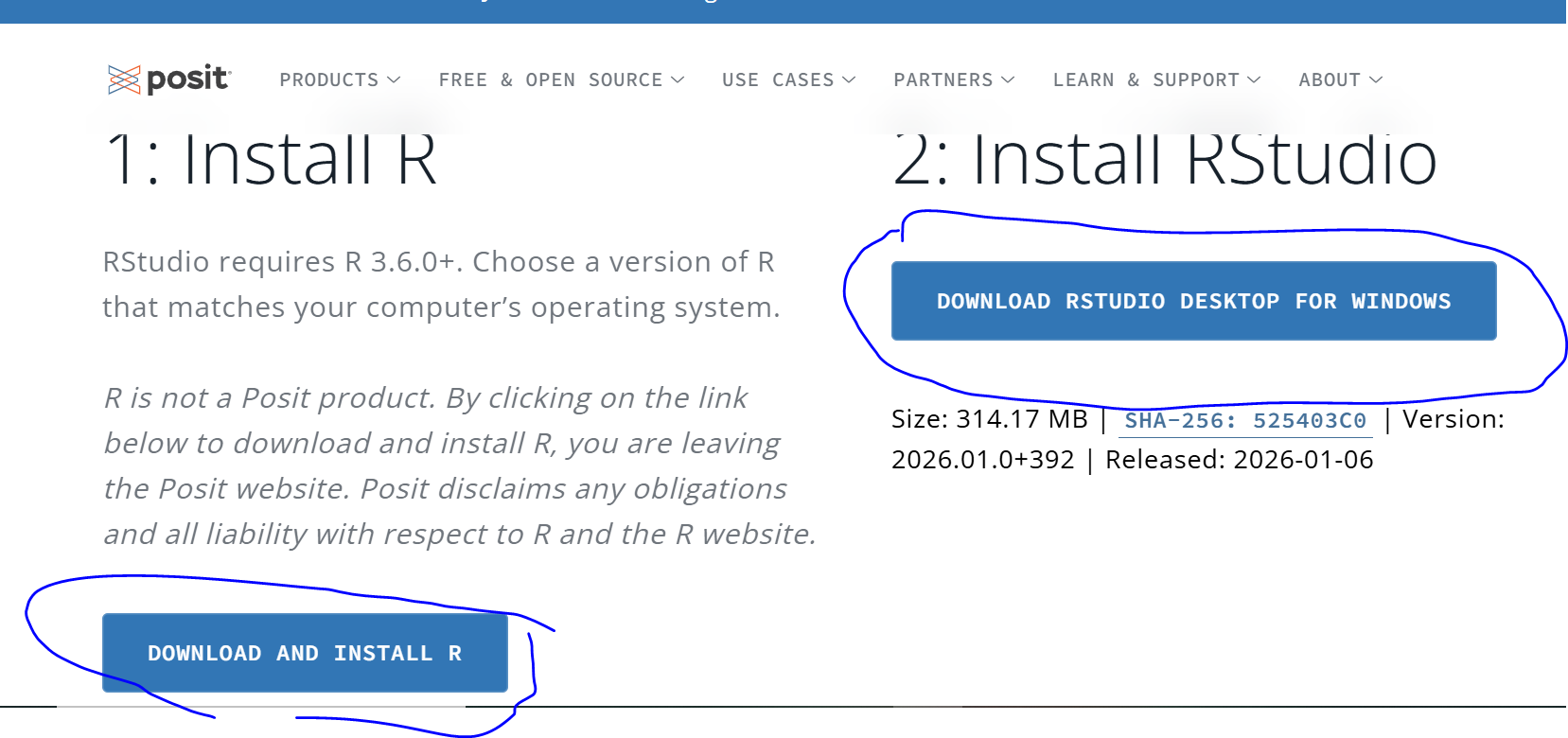
R is currently maintained by a team called the R core team which consists of volunteers and open source enthusiasts. The latest version of R alongside Rstudio editor can be downloaded here: R and Rstudio Download
Figure 2.1: Download R and Rstudio
Once installed you can either write your commands/code in the console or open an editor and write your code there. It is recommended to write in the editor, because this will allow you to save your code as a script for future use. The code you write in the console gets lost the most you exit R.
Comments in R are done using the hash symbol like so #this is a comment
You can use R as a calculator to do basic mathematical computations but you can also use it to do sophisticated analysis that may involve models and graphs. These advanced uses of R are usually enhanced through third party contributed software that comes in the name of packages. An R package is the fundamental unit of share able code. An R package is simply a collection of functions, data, and documentation on how to use those functions. For example to use visualization functions within a package called ggplot we do the following;
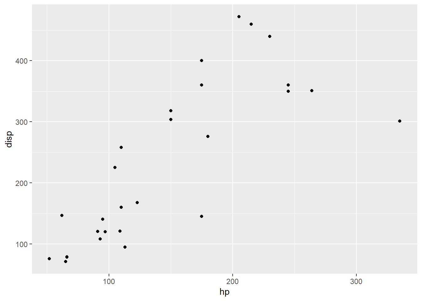
#| warning: false# first install the package if you are using it for the first time.# install.packages('ggplot2') install a package only once but load it # every time you want to use it.# Once installed we only need to load it into our session and we will have# access to the functions and data contained in it. # To load a package we use the function library().library(ggplot2)#use functions in ggplotggplot(mtcars, aes(x = hp, y = disp)) +geom_point()
It’s okay if you don’t understand the code above for generating a scatter plot. The purpose here is to show you how to install, load, and use functions within a package.
2.2 R data types and objects
Just like many other programming languages, R also has the concept of data objects and data types. Data objects can be likened to containers while data types define the nature of the contents of the container.
R has support of various objects, actually almost everything you will encounter in R can be treated like an object. The major data objects you will encounter frequently include; vectors, lists, matrices, arrays, factors, and data frames. Vectors are one-dimensional in nature, the other objects are multi-dimensional. These objects helps us to store data in R, and the nature of the data will dictate the type of the container (object) we use.
Once we have the container, we need to understand the data types that will describe the contents. R comes with five data types; Character, Numeric (integers and floats or doubles), Boolean (trues and false), Complex, and Raw You will rarely use the complex and the raw data types in practice but its good to be a ware of their presence. Creating these data types in R is easy and therefore left as an exercise to the reader. Actually in practice you will rarely create them, but we will find them in rectangular data sets which are presented in R as data frames. Within a data frame you have rows or observations and columns also called variables. These variables will be either be of character type like gender, or numeric like age, or Boolean like responses to a binary question.
As an example, lets create a data frame from scratch and examine the data types of each column.
# start by defining the vectors of interest.age <-c(20,23,41,16,50,11)gender <-c('Male', 'Female','Female','Male','Male','Male')status <-c(TRUE, TRUE, FALSE, FALSE, FALSE, TRUE)dataframe1 <-data.frame(age, gender, status)# examine the structure of our data frame, this will tell us the data type of# each variable/column as well.str(dataframe1)
# we see that age is numeric, gender is character, and status is logical
In the process of making the data frame, you see that to create a vector we use the c() function and list the contents we want separated by commas. We decide on the names of our objects and then bind those names to our data using the assignment operator (<- ).
2.3 Importing data
To do your analysis on clinical trials data, you need to have the data loaded into the R system. There are various ways of getting your data into R and we will look at a few that are common.
The first step is to ensure that your working directory is pointing to where your data is stored. If you are using Rstudio projects then this is not an issue because whenever you create a project from a directory that directory automatically becomes your working directory. In fact, I would like to emphasize that you force yourself to start using Rstudio projects this early in your career or in your academic endeavors. They will prove very useful in the long run. They will also help you avoid using absolute paths in your R scripts.
Reading csv files which are common in practice can be done with a function called read.csv().
# I have a csv file saved in a folder called data which is in the directory# of my Rstudio project. To read it into R I will type the following commandsdata1 <-read.csv("data/diabetes_dataset.csv")head(data1[, c('age','gender','ethnicity','income_level','education_level')])
  age gender ethnicity income_level education_level
1  58   Male     Asian Lower-Middle      Highschool
2  48 Female     White       Middle      Highschool
3  60   Male  Hispanic       Middle      Highschool
4  74 Female     Black          Low      Highschool
5  46   Male     White       Middle        Graduate
6  46 Female     White Upper-Middle      Highschool
The readr package comes with improved functions like read_csv() that can be used instead of the base read.csv() function, we encourage you to explore all the functions within it. Another good package that you will encounter is haven, this is mostly used to read data from other statistical systems like SAS, STATA, and SPSS please take time to explore this package as well. To import Excel workbooks into R we use the readxl package with the function read_excel().
2.4 Introduction to the tidyverse
The modern way of programming in R has evolved in recent times to conform to the concepts of tidy data and the philosophy employed in the tidyverse ecosystem. This philosophy was initially engineered by Hadley Wickham chief scientist at Posit Studio but it’s currently being worked on by several other developers/scientists.
A collection of libraries form part of the tidyverse package. These libraries include ggplot2, dplyr, lubridate, forcats, stringr, readr among others. Using these collection you can conduct a lot of modeling and visualization to your data. The dplyr package for example gives you the necessary tools you need to wrangle your data. You get a grammar of data manipulation, where you can perform various verbs like selecting columns, filtering rows, creating new columns, and performing summaries on grouped data. The ggplot2 package gives you the grammar of data visualization.
The functions in the tidyverse packages can be used together in a sequence using a special operator called the pipe. The pipe operator allows one to write a pipeline that outline a sequence of related steps. There are two types of pipes allowed in R, namely the base pipe operator ( |> ) and the magrittr pipe (%>%). In this book we shall use the base pipe operator because its freely available in R versions 4.1 and above. The magrittr operator is only available after loading the magrittr package.
Let’s see all of these in action in the below code chunk.
# install the tidyverse package if not yet installed# install.packages("tidyverse")library(tidyverse)# we can now select a few columns in the mpg data set and perform# some filtering.# and even create a new column based on existing columns.mpg |> dplyr::select(manufacturer , model, displ, year, hwy) |> dplyr::filter(manufacturer =='nissan') |> dplyr::mutate(dipl2 = displ *2)
#perform a summary; get average displacement per manufacturermpg |> dplyr::group_by(manufacturer) |> dplyr::summarise(mean =mean(displ))
# A tibble: 15 × 2
   manufacturer  mean
   <chr>        <dbl>
 1 audi          2.54
 2 chevrolet     5.06
 3 dodge         4.38
 4 ford          4.54
 5 honda         1.71
 6 hyundai       2.43
 7 jeep          4.58
 8 land rover    4.3
 9 lincoln       5.4
10 mercury       4.4
11 nissan        3.27
12 pontiac       3.96
13 subaru        2.46
14 toyota        2.95
15 volkswagen    2.26
We will use this programming style in the rest of this book so its important for you to get familiar with it to enjoy the rest of this book’s content.
2.5 Handling of missing values
Missing values are ubiquitous with real world data, and so it’s important we know how to handle them. The is.na() function is your best friend in R for detecting missing values. Missing values in R are represented by the sentinel NA which means not a applicable or not a number. If you perform a computation on a vector that has some missing values you will get NA as the result. To specify to the function that you want to carry out your computation on only non-missing data, you use the na.rm = True argument.
SAS data sets that you will encounter a lot in clinical trials may come with missing values in form of blanks. We need to tell R to explicitly convert these blanks to NA(Not A Number/Not Applicable) values. We will see how to do that in ADAMs chapter using the admiral package. Whether you should delete or impute missing values is something that will be mentioned by the clinical trial statisticians in a special document called the Statistical Analysis Plan (SAP).
2.6 Basics of data visualization
As a statistical programmer you will encounter a number of graphs in your work, therefore it’s imperative that you familiarize yourself with how to create them using the R language. There are so many systems for creating graphs ranging from Base R functions to functions provided through third party packages like lattice and ggplot2. In most cases you will be creating or interacting with graphs created using the ggplot2 system which is an implementation of the grammar of graphics. Once you have mastered ggplot2 you can explore other systems like plotly for creating interactive graphs and rshiny for creating entire visualization apps.
2.6.1 An overview of ggplot2
ggplot2 is an R package developed by Rstudio Chief Scientist Hadley Wickham. With ggplot we can create a wide variety of graphs using a unified programming style. This style follows a layered approach where we create a complete graph by combining various layers. We only to specify three components to have a complete graph, the first one is data, then followed by aesthetics that map our data to the y and x axis of our graph and finally we need to specify the geometric shape we need eg points or lines. Let’s look at a few examples;
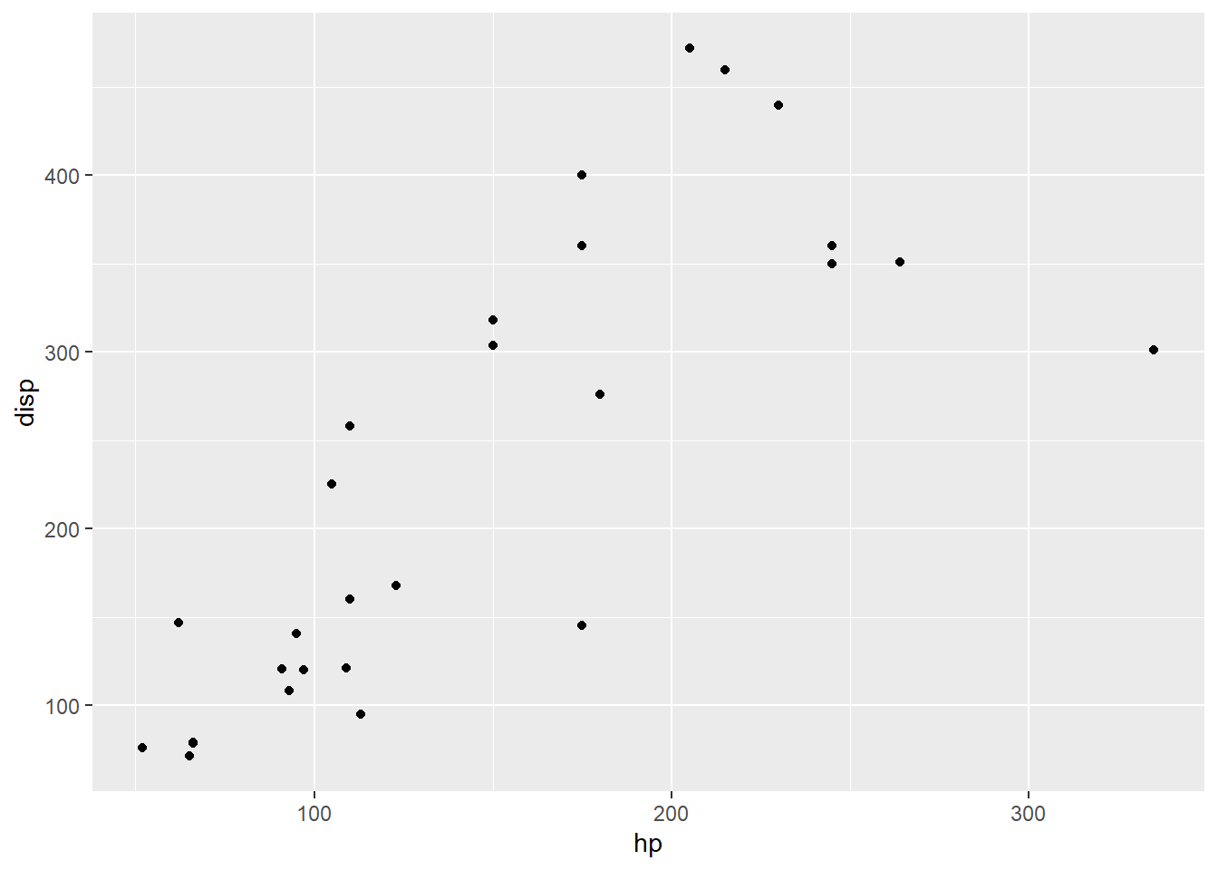
library(ggplot2)ggplot(data = mtcars, #specify the data you want to plotmapping =aes(y = disp, x = hp)) +# specify the mappinggeom_point() # then finally specify the geometric shape you need
This is the most basic plot that we get with ggplot code. We can keep on adding other layers like labels and themes to improve the overall look. There are so many geoms (geometrical objects) available, please explore them in the ggplot2 documentation online.
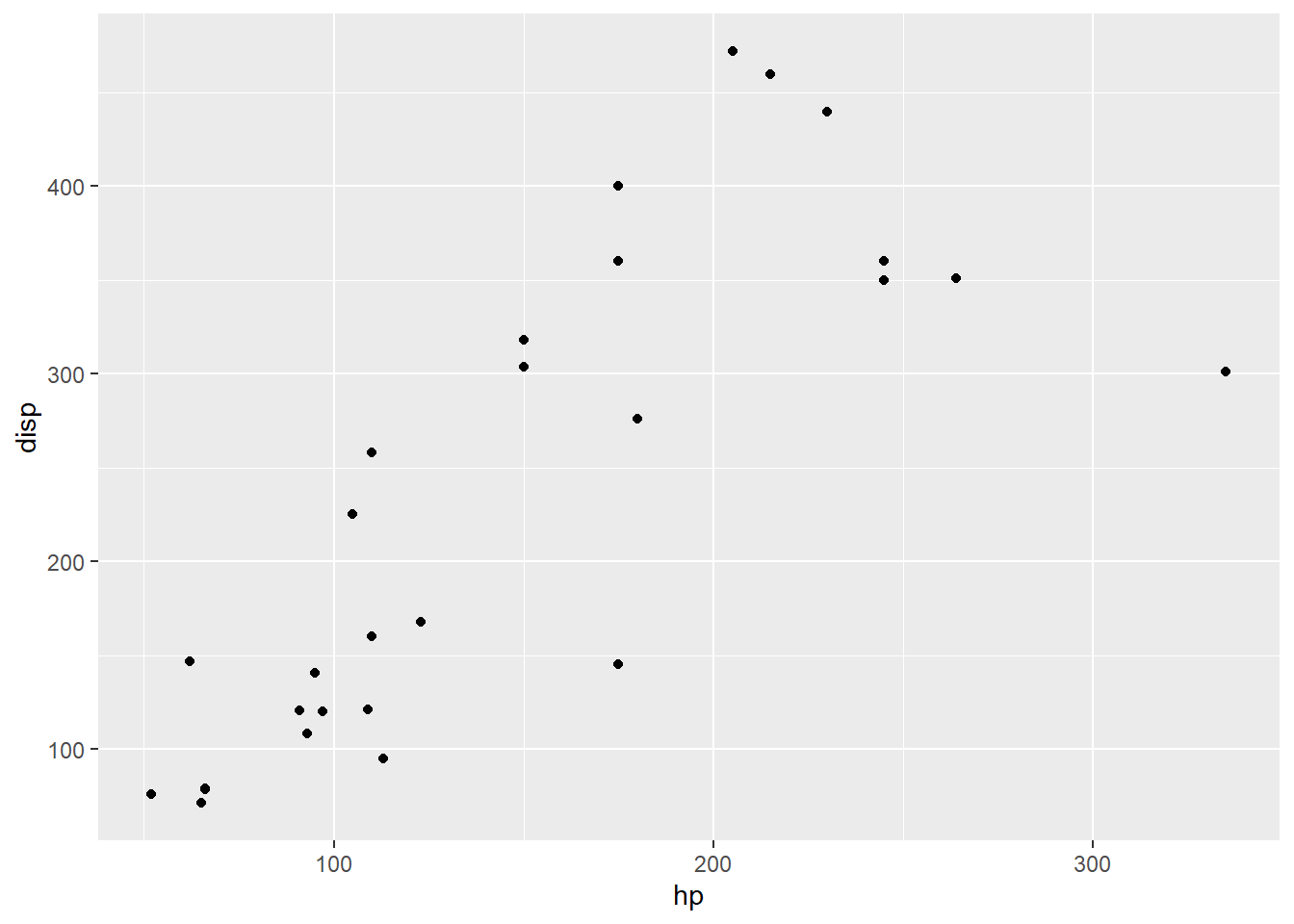
Because almost every ggplot call will contain data and mapping, we don’t have to specify these arguments by name, we can shorten the above code as below;
ggplot(mtcars, aes(y = disp, x = hp)) +geom_point()
2.7 Basics of modeling
Modeling is part and parcel of what we do as statisticians/programmers/data scientists in our day to day work. This section is just an overview of how to conduct statistical modeling in R. The common functions that you will use in R to carry out modeling are lm() and glm(). lm is for linear modeling, you will use this to fit both simple and multiple linear regression models, while glm is for fitting generalized linear models like logistic regression, Poison regression etc.
broom and gtsummary packages will help you display nice regression output tables ready for publication, we will illustrate how to use them in the below examples.
2.7.1 Some examples
2.7.1.1 Linear models
These are divided into two, simple linear regression that has only one independent variable and multiple linear regression that has more than one independent variables.
library(broom)library(gtsummary)model1 <-lm(mpg ~ disp, data = mtcars)model1 |> broom::tidy() |> knitr::kable(caption ='Simple Linear Regression')
Simple Linear Regression
term
estimate
std.error
statistic
p.value
(Intercept)
29.5998548
1.2297195
24.070411
0
disp
-0.0412151
0.0047118
-8.747151
0
model1 |>
  gtsummary::tbl_regression()
Characteristic
Beta
95% CI
p-value
disp
-0.04
-0.05, -0.03
<0.001
Abbreviation: CI = Confidence Interval
model2 <-lm(mpg ~ disp + hp + drat + wt + qsec, data = mtcars)model2 |> broom::tidy() |> knitr::kable(caption ='Multiple Linear Regression')
Multiple Linear Regression
term
estimate
std.error
statistic
p.value
(Intercept)
16.5335696
10.9642303
1.5079553
0.1436221
disp
0.0087202
0.0111891
0.7793462
0.4428123
hp
-0.0205981
0.0152831
-1.3477698
0.1893597
drat
2.0157746
1.3094595
1.5393944
0.1357912
wt
-4.3854639
1.2434321
-3.5269026
0.0015841
qsec
0.6401499
0.4593443
1.3936166
0.1752327
model2 |>
  gtsummary::tbl_regression()
Characteristic
Beta
95% CI
p-value
disp
0.01
-0.01, 0.03
0.4
hp
-0.02
-0.05, 0.01
0.2
drat
2.0
-0.68, 4.7
0.14
wt
-4.4
-6.9, -1.8
0.002
qsec
0.64
-0.30, 1.6
0.2
Abbreviation: CI = Confidence Interval
2.7.1.2 Generalized Linear Models
When the dependent variable does not follow the Normal Distribution, but follows some other distribution like the Binomial Distribution, then we need a general class of models to model this type of a variable. This leads to generalized linear models. Let’s look at an example of Logistic regression model which is common in modeling binary outcomes like survival on the titanic.
# We need to tell R that our outcome variable is a factor variabledataset$Survived <-as.factor(dataset$Survived)# lets convert character columns into factor variablesdataset$Sex <-as.factor(dataset$Sex)dataset$Embarked <-as.factor(dataset$Embarked)dataset$Pclass <-as.factor(dataset$Pclass) # this variable has only three distinct values and therefore we can model it as categorical instead of numericglm1 <-glm(Survived ~ Age + Sex + Embarked + Pclass + Fare + SibSp,data = dataset,family =binomial(link ='logit'))glm1 |>tbl_regression(exponentiate =TRUE)
Characteristic
OR
95% CI
p-value
Age
0.96
0.94, 0.97
<0.001
Sex
female
—
—
male
0.07
0.05, 0.11
<0.001
Embarked
C
—
—
Q
0.44
0.13, 1.41
0.2
S
0.67
0.39, 1.14
0.14
Pclass
1
—
—
2
0.30
0.16, 0.57
<0.001
3
0.09
0.05, 0.17
<0.001
Fare
1.00
1.00, 1.01
0.6
SibSp
0.68
0.53, 0.87
0.002
Abbreviations: CI = Confidence Interval, OR = Odds Ratio
2.8 Getting help when stuck
We all get stuck at some point in our learning endeavors and knowing how to find your way out is one of the top skills one has to develop. In R whenever you are stuck on how to use a certain function simply type help(function name) in the console or ?function name. This will pull up the documentation for that particular function in the viewer pane where you can learn about all its arguments and you get to see some examples of the function in practice.
When you get an error, simply copy the error and paste it online. In most cases, you will find that someone else experienced a similar issue before and they were kind enough to post the solution online. You can also post your error or question on stack overflow, but please remember to read their code of conduct first lest you annoy people by asking something that has already been addressed.
2.9 Learning more
To have a deeper knowledge of R I recommend the following books where you will learn the essential programming skills applied to various kinds of data. None of these will teach you something specific to clinical trials but reading them will help you understand quickly the R code that is specifically used in clinical programming.